This describes how I have implemented my own neural network. The article focuses mainly on the math and calculations, in order to save somewhere the know how and how I did it.

This is sub-layout for documentation pages

Top

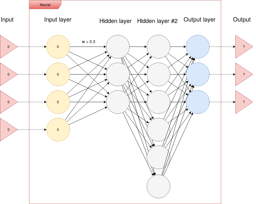
Neural network can be seen as a multivariable function. We give it multiple inputs, and we get multiple outputs.

The neural network we will be discussing here, is neural network, which has one input layer, \(n \in <2, \inf>\) hidden layers, and one output layer.
Here is an illustration of such a neural network:

2.1 Definitions

Let's start with some axioms (or definitions), to have some naming convention we can use.
Note: These definitions are defined by me, and do not necesarrily have to apply to all existing implementations of neural networks that exist in the world, but they apply to my implementation precisely!

• Neural network contains \(n \in <2, \inf>\) layers (indexed from 0), where first layer \(L_0\) is the input layer, the last layer \(L_n\) is the output layer, and other layers are called hidden layers (if any)
• Layer \(L\) contains \(<1, \inf>\) nodes (or neurons) \(N\)
• Node \(N\) from layer \(L\) is only connected to all nodes in layer \(L + 1\), if such layer exists.
• weight \(w\) is any connection between any two nodes \(N_1\) \(N_2\). This weight has a numeric, decimal value \(<-1, 1>\)
• bias \(b\) is a numeric, decimal value \(<-1, 1>\), which is assigned to all nodes, with exception of nodes that are in the input layer
• \(W_{i,i+1} \in M\) is a matrix of weights between layers \(L_i\) and \(L_{i+1}\)
• \(\Delta w_{i-1,i}\) is a matrix telling how to alter the weights \(W_{i-1,i}\), mentioned above
• \(B_i \in M_{x,1}\) is a matrix of biases for layer \(L_i\), \(x\) is amount of nodes in layer \(L_i\)
• \(\Delta b_i\) is a matrix telling how to alter the biases \(B_i\), mentioned above

2.2 Feed forward

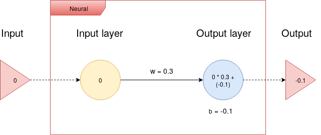
Informally, feed forward is an operation, which takes an input, and pulls it through the neural network to generate an output.

Let's imagine one input and one output neuron, then, the output calculation is shown by the following illustration:

So, what we need to calculate for each layer are two values, \(\Delta w\) and \(\delta b\)
\(\Delta w\) tells, how we have to alter weights going into the currenlty processed layer, with respect to the error.
\(\delta b\) tells, how we have to alter biases for all nodes of the currenlty processed layer, with respect to the error.
(understanding, that we never calculate back propagation for the input layer \(L_1\))

4.1 Definitions

In order to unwrap this complex math topic, let's start with some definitions:

• Let \(a(x)\) be an activation function of the neural network, in this case, \(a(x)=\frac{1}{1+e^{-x}}\) is the sigmoid function
  Then, the first derivative is \(a^\prime(x) = x*(1-x)\) ( as can be seen here)
• Let \(G(M)\) be a function, which applies function \(a^\prime(x)\) on each element \(e\) of an input matrix \(M\)

Then for calculation of the \(\Delta w_{i-1,i}\) for weights between layers \(i-1\) to \(i\) applies:
\(\Delta w_{i-1,i} = l_r * (G(O_i) \circ E_i) * O_{i-1}^\top\)
where

• \(\circ\) is the Hadamard product upon matrices
• \(*\) is the matrix multiplication operation, if the adjacent elements are matrices / vectors
• \(l_r \in \!R\), \(l_r > 0\) is the learning rate
• \(O_{i} \in M_{n,1}\) is the output from layer \(L_{i}\). Applies \(i \in <1,n>\)
• \(E{i} \in M_{n,1}\) is the error from layer \(L_{i+1}\). For \(E_n\) applies \(E_n = O_n - expected\), where \(O_n\) is the output from the output layer and \(expected\) is the known corect result, we expect

For calculation of the \(\Delta b_i\) for layer \(L_i\) applies:
\(\Delta b_i = l_r * (G(O_i) \circ E_i) \)
where the constants are the same as the ones explained above

For \(E_i\), where \(i \neq n\) (is not output layer), applies:
\(E_i = (W_{i,i+1} + \Delta w_{i,i+1})^\top * E_{i + 1}\)

Because, from experience, it is easier to understand someting from example, than from bunch of definitions, here is calculated example.
Let's have following neural network:

Assume, that we are using the sigmoid function as an activation function:
\(a(x)=\frac{1}{1+e^{-x}}\)
Let's define, that learning rate \(lr=0.1\)
Let's now do step by step the entire back propagation.
We will label layers as \(L_1\) (input),\(L_2\) (hidden #1),\(L_3\) (hidden #2), \(L_4\) (output)

First, we will run feed forward, and we will remember all output matrices \(O_1\),\(O_2\),\(O_3\),\(O_4\), where
\(O_1\) is the output from \(L1\) (so the plain input)
\(O_2\) is the output from \(L2\)
\(O_3\) is the output from \(L3\)
\(O_4\) is the output from \(L4\) (so the final output of the network)

We see from the picture, that \(O_4 = \begin{bmatrix}0.4759\\0.5413\\0.6256\end{bmatrix}\)

If we would calculate feed forward, we would get the output matrices for each layer (here, calculated by the neural network itself..)
\(O_1 = \begin{bmatrix}0\end{bmatrix}\) \(O_2 = \begin{bmatrix}0.7310\\0.4501\\0.5744\end{bmatrix}\) \(O_3 = \begin{bmatrix}0.5938\\0.3386\end{bmatrix}\)

The weight matrices (weights between the layers, written to a matrix) are:
\(W_{1,2} = \begin{bmatrix}0.3\\-0.1\\0.2\end{bmatrix}\) \(W_{2,3} = \begin{bmatrix}0.4 & 0.1 & -0.1\\0.1 & 0.1 & -0.5\end{bmatrix}\) \(W_{3,4} = \begin{bmatrix}0.4 & -0.1\\-0.4 & 0.6 \\ -0.2 & -0.2\end{bmatrix}\)
The bias matrices for all layers are:
\(B_{1} = undefined\) \(B_{2} = \begin{bmatrix}1\\-0.2\\0.3\end{bmatrix}\) \(B_{3} = \begin{bmatrix}0.1\\-0.5\end{bmatrix}\) \(B_{4} = \begin{bmatrix}-0.3\\0.2'\\0.7\end{bmatrix}\)

Then, we start processing the layers, from \(L_4\) to \(L_1\)

5.1 Processing \(L4\)

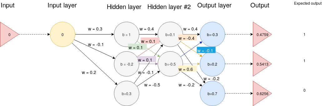
The actual network weight matrix between layers \(L_3\) and \(L_4\) is \(W_{3,4}\)
We need to calculate \(\Delta W_{3,4}\), for which applies the equation above

Error from output \(E_4\) is expected result - \(O_4\), because \(L_4\) is the last layer
\(E_4 = \begin{bmatrix}1\\1\\0\end{bmatrix} - \begin{bmatrix}0.4759\\0.5413\\0.6256\end{bmatrix}= \begin{bmatrix}0.5241\\0.4587\\-0.6256\end{bmatrix} \)

Gradient \(G(O_4)\) results in

\( G(O_4) = \begin{bmatrix}0.1966\\0.2475\\0.2444\end{bmatrix} \)

Therefore \(\Delta w_{3,4}\) is

\(\Delta w_{3,4} = l_r * (G(O_4) \circ E_4) * O_3^\top \)
\( = 0.1 * ( \begin{bmatrix}0.1966\\0.2475\\0.2444\end{bmatrix} \circ \begin{bmatrix}0.5241\\0.4587\\-0.6256\end{bmatrix} ) * \begin{bmatrix}0.5938 & 0.3386\end{bmatrix} \)
\(= \begin{bmatrix}0.0077 & 0.0044\\0.0067 & 0.0038\\-0.0087 & -0.0049\end{bmatrix} \)

We will then add \(\delta w_{3,4}\) to \(W_{3,4}\)

\(\Delta b_4 = l_r * (G(O_4) \circ E_4) \)
\(= 0.1 * ( \begin{bmatrix}0.1966\\0.2475\\0.2444\end{bmatrix} \circ \begin{bmatrix}0.5241\\0.4587\\-0.6256\end{bmatrix} ) = \begin{bmatrix}0.0130\\0.0113\\-0.0146\end{bmatrix} \)
We will then add \(\Delta b_4\) to \(B_4\)

5.2 Processing \(L3\)

Error from output \(E_3\) is
\(E_3 = (W_{3,4} + \Delta w_{3,4})^\top * E_4\) \(= (\begin{bmatrix}0.4 & -0.1\\-0.4 & 0.6 \\ -0.2 & -0.2\end{bmatrix} + \begin{bmatrix}0.0077 & 0.0044\\0.0067 & 0.0038\\-0.0087 & -0.0049\end{bmatrix})^top * \begin{bmatrix}0.5241\\0.4587\\-0.6256\end{bmatrix} = \begin{bmatrix}0.1638\\0.3551\end{bmatrix} \)

Gradient \( G(O_3) = \begin{bmatrix}0.2411\\0.2239\end{bmatrix} \)

Therefore
\(\Delta w_{2,3} = l_r * (G(O_3) \circ E_3) * O_2^\top \)
\( = 0.1 * ( \begin{bmatrix}0.2411\\0.2239\end{bmatrix} \circ \begin{bmatrix}0.1638\\0.3551\end{bmatrix} ) * \begin{bmatrix}0.7310 & 0.4501 & 0.5744\end{bmatrix} \)
\(= \begin{bmatrix}0.0028 & 0.0017 & 0.0022\\0.0058 & 0.0035 & 0.0045\end{bmatrix} \)

We will then add \(\delta w_{2,3}\) to \(W_{2,3}\)

\(\Delta b_3 = l_r * (G(O_3) \circ E_3) \)
\(= 0.1 * ( \begin{bmatrix}0.2411\\0.2239\end{bmatrix} \circ \begin{bmatrix}0.1638\\0.3551\end{bmatrix} ) = \begin{bmatrix}0.0039\\0.0079\end{bmatrix} \)

5.3 Processing \(L2\)

Error from output \(E_2\) is
\(E_2 = (W_{2,3} + \Delta w_{2,3})^\top * E_3\) \(= (\begin{bmatrix}0.4 & 0.1 & -0.1\\0.1 & 0.1 & -0.5\end{bmatrix} + \begin{bmatrix}0.0028 & 0.0017 & 0.0022\\0.0058 & 0.0035 & 0.0045\end{bmatrix})^top * \begin{bmatrix}0.1638\\0.3551\end{bmatrix} = \begin{bmatrix}0.1036\\0.0534\\-0.1919\end{bmatrix} \)

Gradient \( G(O_2) = \begin{bmatrix}0.1966\\0.2475\\0.2444\end{bmatrix} \)

Therefore
\(\Delta w_{1,2} = l_r * (G(O_2) \circ E_2) * O_1^\top \)
\( = 0.1 * ( \begin{bmatrix}0.1966\\0.2475\\0.2444\end{bmatrix} \circ \begin{bmatrix}0.1036\\0.0534\\-0.1919\end{bmatrix} ) * \begin{bmatrix}0\end{bmatrix} \)
\(= \begin{bmatrix}0\\0\\0\end{bmatrix} \)

We will then add \(\delta w_{1,2}\) to \(W_{1,2}\)

\(\Delta b_2 = l_r * (G(O_2) \circ E_2) \)
\(= 0.1 * ( \begin{bmatrix}0.1966\\0.2475\\0.2444\end{bmatrix} \circ \begin{bmatrix}0.1036\\0.0534\\-0.1919\end{bmatrix} ) = \begin{bmatrix}0.0020\\0.0013\\-00046\end{bmatrix} \)

Congratulations, we have successfully finished the back propagation of the neural network
The wolfram mathematica notebook with these calculations can be downloaded here